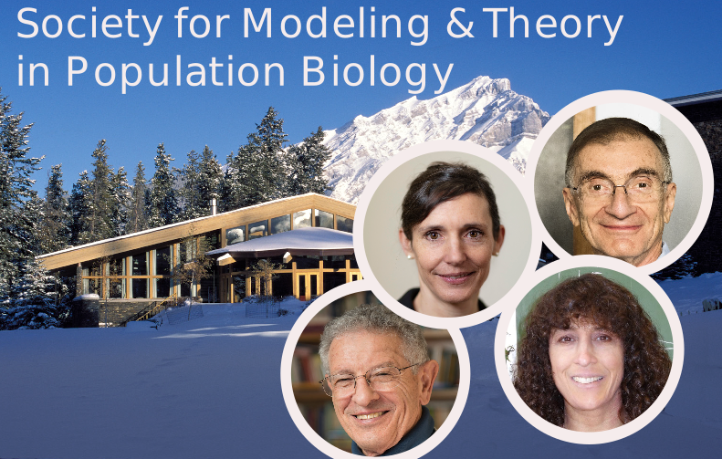
The January 11, 2024 kickoff event of the Modeling & Theory in Population Biology series featured four speakers: Maria Servedio from the University of North Carolina, Marc Feldman from Stanford, Joel E. Cohen from Rockefeller University, and Tanja Stadler from ETH Zürich. This group of speakers reflected the initial inspiration for this program: how diverse problems within the field of population biology can be investigated using some of the same techniques. Our discussion spanned evolution to epidemiology and beyond. Plus, this event provided a unique platform for speakers to get into the details of the modeling and theory that supported their research that might otherwise be glossed over in venues of a less specialized audience.

Maria Servedio – “The role of theory in evolutionary biology”
Our first speaker, Maria Servedio, spoke to the role of theory in evolutionary biology and ecology – identifying theory as a set of techniques that can apply to many interests and goals, despite remaining a minority within biology.
Servedio framed her discussion with an illustration of several continua along which scientists might place their studies: specific to abstract, quantitative to qualitative, and descriptive to proof of concept, providing examples of each. Addressing the group, Servedio said, “We can probably take our own studies and place a dot for each study on each of these lines as to where we would think it would fall, and as theoreticians, we have an appreciation for studies that are scattered throughout these continua. But I’m going to spend a little bit more time talking about this far right of the continuum [referring to abstract, qualitative, and proof of concept studies], because I found that studies that fall here are especially hard to communicate to empiricists. This can be particularly true if you’re talking to a broad-based biology department, which, of course, is going to happen.”
She drew from her early experience as an assistant professor working on the effects of sexual imprinting to illustrate why better strategies to communicate theoretical work are necessary. In this example, she wanted to understand the evolutionary forces acting on and generated by different types of sexual imprinting, so allowed 3 empirically supported types of imprinting to evolutionarily compete in her model: maternal, paternal, and oblique imprinting.
Maternal imprinting involves the choosing sex acquiring a mating preference by imprinting on the phenotype of their mother. This becomes the trait that they prefer in mates. Paternal imprinting works similarly, but via imprinting on the father. Oblique imprinting involves the juvenile imprinting on the adults in a population in proportion to the phenotypes that they encounter.
Exploring these types of imprinting meant creating a haploid phenogenotypic model, then competing 2 types of imprinting strategies at a time. She and her colleagues found that whenever paternal is in one of these competitions, it fixes, whereas in maternal and oblique strategies, the result depends: if there’s no viability selection, there’s no evolution, meaning these strategies are completely neutral. However, if there’s viability selection favoring the more common trait, maternal fixes.
“Our goal wasn’t really to show what happened, but to understand the evolutionary forces involved,” Servedio explained about these experiments, “and this is one thing I really love about theory… you can get at these why questions by digging in a little bit more, and I love doing that part.”
They encountered two properties that could help them understand these results: the first was the property of the “imprinting set,” which is a term coined for the paper, defined as a set of all individual uses of a template for imprinting, given a particular imprinting strategy. In other words, the set of individuals that are imprinted upon.
The oblique imprinting set, for example, will be all of the adults or all of the males. Considering all the adult phenotypes, there will be a one-to-one mapping with the oblique imprinting set. It will consist of all surviving members of the previous generation, assuming females and males have equal frequencies. The maternal and oblique set will be the same as each other if all females have equal mating success.
The paternal imprinting set works differently in that females don’t imprint on all of the males in the previous generation. They only imprint on the fathers, so that they only imprint on males that are successfully mated. So, the paternal set is impacted by sexual selection, and this causes a big difference. With this, it’s evident that which imprinting strategy will evolve depends on the answer to the question: which strategy’s imprinting set has a higher frequency of the more fit trait?
Servedio and colleagues found the fitter trait to appear with the highest proportion in the paternal set, making this the set with the highest fitness over the maternal and oblique sets. This is because imprinting causes positive frequency-dependent sexual selection, and this will be stronger if there is more of a skew in the frequencies initially, generating a more common preference for the more successful trait. When using the paternal set, this also ultimately benefits the allele that causes a female to paternally imprint. One can predict that paternal imprinting should outcompete peer-to-peer, which should outcompete maternal. Servedio’s research team found exactly this to be the case when tested. They found the property of imprinting sets to be interesting in that it explained why paternal imprinting fixed. However, it didn’t explain why, when you add in viability selection, maternal imprinting should win over oblique, because they had the same imprinting sets. This told the researchers that something else also had to be going on.
They continued investigating and found that the other affecting property was the phenogenotypic disequilibrium that was established in the system. Phenogenotypic disequilibrium is the same as linkage disequilibrium except that it is between a stored phenotypic information unit and trait allele. Phenogenotypic disequilibria are generated anew each generation during imprinting.
The research team calculated an internal pairwise phenogenotypic disequilibrium between the preference and the trait within each imprinting set. This was positive when maternal imprinting was present, because individuals prefer their mother’s phenotype, which they’re likely to have inherited.
It was zero with oblique imprinting, because individuals’ traits have no relationship to the preference they acquire as they’re imprinting on unrelated adults.
This culminates in giving an advantage to maternal imprinting in a way which the researchers were able to track with math, and it also accounts for exceptions to the rule. So when viability selection favors the rarer trait, thinking about and understanding phenogenotypic disequilibrium explains why, in that case, oblique imprinting fixes.
Servedio recalled feeling satisfied for having set out and accomplished her goal of understanding the forces involved in the evolution of these strategies, so the question that succeeded her tenure talk took her by surprise. It came from a developmental biologist who asked how one might test this model in Drosophila – a question that seemed to demonstrate a misunderstanding of the proof of concept model, whose capacities were not clear to those accustomed to empirical studies.
Partially inspired by this experience amongst others, Servedio with several junior colleagues published a “full-throated defense” of proof of concept models in PLOS Biology in 2014: “Not Just a Theory – The Utility of Mathematical Models in Evolutionary Biology.” They compared empirical and proof of concept approaches as ways of applying the scientific method, and pointed out that proof of concept models carried out the scientific method by using math to test links and verbal chains of logic, from an initial hypothesis to conclusions.
Servedio explained that a more constructive way to ask “How would you test your model?” is “How would you test your assumptions empirically?” If one tests the predictions of a model and finds them unmet after having done the math correctly, what it really means is that there are some assumptions that were not made.
The onus of improving theory literacy is on theorists – Servedio learned from her experience and now starts her talks with analogies between proof of concept models and empirical models if speaking to a mixed audience. She notes that theorists ought to be aware that non-theoriticists may “glaze over” the math portions of a presentation, and recommends being conscious of the quantity and detail of mathematical content in order to keep information accessible.
She also touched on a survey she performed in 2020, asking 8 ecologists and 16 evolutionary biology theorists to classify 10 citations to one of their papers as incorrect or “correct but general” (rather than specific to their study). This resulted in an average of 20% incorrect citations, and up to 40% for one paper. The more abstract papers tended to have more incorrect citations, while the quantitative papers were generally more correct.
Servedio’s talk culminated with two calls to action for the scientific community: for theorists to better communicate how theory plays a role in biology in a way that empirical biologists can understand, and for there to be a greater dissemination of theory in biology classrooms. Servedio looked forward to the Society for Modeling and Theory in Population Biology becoming “a community where we can appreciate each other’s work, where we can advocate for other scientists who are using theoretical techniques, and where we can find ways to increase the appreciation that non-theoreticians have for theoretical work.”

Marc Feldman – “Reflections on Theoretical Population Biology then and now”
Having served as the managing editor for 41 years, no one other than Dr. Marc Feldman could be better positioned to present “Some reflections on the journal Theoretical Population Biology.”
He began with the story of how the journal came about: in 1969, his thesis advisor Samuel Karlin suggested that there was not enough scope in the current biology journals to support growth in theoretical population biology, and that a new journal specializing in the field was needed. Feldman, having just finished his PhD, agreed to become managing editor of this new journal.
Feldman pointed out that the journal was not the first time that theory was incorporated into population biology. A Short History of Mathematical Population Dynamics by Nicolas Bacaër presents a long list of instances in which theory had been included in issues of population: early life tables, foundations of what we think of as epidemiology, branching processes, early papers on theoretical ecology, and more.
Moving on to Stanford’s particular connection to theoretical population biology, Feldman described Walter Bodmer, a former student of R. A. Fisher, arriving to the newly formed genetics department in the medical school and meeting Samuel Karlin and Jim McGregor. Through their conversations, particularly around P. A. P. Moran’s 1958 paper “Random processes in genetics,” it became clear to Karlin that there was scope within the field of genetics for more formal and applied mathematics. The first real new contribution that Karlin and McGregor made to population genetics was the introduction of direct product branching processes, the origins of which can be traced to Moran’s book Statistical Processes of Evolutionary Theory.
When they proceeded to apply some of these approximations to the stochastic processes that underlay the work of Fisher and Wright, they showed that there were different classes of diffusion models that could be developed under different assumptions on the relationship between the parameters and the population size. It was rather unpopular at that time, especially given that there was kind of an antipathy towards mathematics at the time. Feldman noted his belief that Theoretical Population Biology as a journal was responsible for the incorporation of mathematics into mainstream evolutionary theory.
He then reviewed some developments in the 1960s that foreshadowed the formation of the journal. Firstly, there simply weren’t enough outlets for the more mathematical papers even as the subject continued to be explored. Quasi-linkage equilibrium was being touted as a way to rescue adaptive topographies, and the ecological work that was initiated by MacArthur and Levins hadn’t yet made it out of the fringes. There was an expansion into demography; for example, questions started to be asked about how you extend demography to take care of the fact that there are two sexes in human populations. The discovery of massive amounts of genetic variation in natural populations in the mid-1960s also demanded an explanation. Finally, there were the beginnings of early computation – although computers were simple and not very capable then, this is when people were starting to use them.
Many eminent people were interested in having their work exposed in Theoretical Population Biology: M S. Bartlett (statistician) was one of the early publishers in the journal, along with Paul Samuelson (economist), Leo Goodman (statistician), Nathan Keyfitz (demographer), Robert MacArthur (founder of modern theoretical ecology), and Kenneth Cooke (mathematical epidemiologist).
Karlin had given Feldman a problem in 1960: he didn’t understand a paper that Masatoshi Nei had published in Genetics, and asked Feldman to explain it. Feldman spent the next five years trying to understand it, and came up with what became the foundations of modifier theory, which was published in Theoretical Population Biology. It showed that under a multi-locus model, genes that cause reduction in recombination rates would succeed. That was a very particular kind of selection model. Feldman went on to give his student Lee Altenberg the problem to find out why it was, mathematically, that there was a reduction principle.
Altenberg made quite a bit of progress in his thesis. However, solving it took until 2017, when Feldman and Liberman applied a theorem of Karlin in a paper that Karlin called “Classifications of selection and migration structures.” That paper had a theorem on reduction of the eigenvalues of certain classes of matrices that Donsker and Varadhan had studied in variational theory, and they were able to use that to show that all of the models that Feldman had worked on earlier on reduction of mutation, migration, and recombination fitted within one mathematical framework.
Feldman and Cavalli-Sforza also developed the beginnings of cultural evolutionary theory, and in the first few papers there were no outlets for this work; Feldman notes that it could not have been published in anthropology journals. The very first paper to analyze simultaneous evolution of genes and culture in 1976, with the foundation of gene culture and coevolutionary theory – that, too, could not have been published in other journals.
Other ideas that came out of Theoretical Population Biology included: evolution of frequency-dependent cultural transmission, which included oblique and horizontal transmission, expanding the theory that Cavalli-Sforza and Feldman had introduced in the seventies, and the notion of gene-culture disequilibrium.
Feldman took a moment to highlight the most recent paper currently in press with his PhD student, Kayla Denton, which incorporates randomness into these cultural transmission models in a way that’s never been done before, and in particular, with respect to conformity.
He pointed out another piece of history that he finds particularly fascinating: “Balanced Polymorphisms with Unlinked Loci” by Moran, published in 1963. Moran wanted to know how many equilibria there were in a two-locus model, and how many could be stable. He claimed at most 5 equilibria and at most 3 could be stationary states. He published it in Australian Journal of Biological Sciences, but Feldman supposes it would have been a great fit for Theoretical Population Biology, had it existed then.
Moran made this claim because Wright thought that evolutionary change could be summarized as populations moving so as to maximize the mean fitness; that is, the notion of adaptive topography. Moran withdrew that 1963 paper, and Feldman quoted his reasoning as follows: “Using this incorrect theory, I attempted to discuss this problem, and how many of these equilibria could be stable. However, the theory is incorrect, and the number of possible stationary and stable points is an open question. It is possible, though, that 5 and 3 are the correct bounds, and this is suggested by the following argument…”
That argument had historic interest to Karlin and Feldman, because when they came up with that two-locus model that was published in the very first issues of Theoretical Population Biology, they showed that there could be 7 equilibria, and that many of them could be stable. Feldman recalls him being initially resistant to the notion, insisting that equilibria have to be the stationary points of the adaptive topography. It took a long time and “a lot of stuff on the blackboard,” Feldman remembers, to convince him that that wasn’t the case.
At the time, how many equilibria and how many could be stable was not generally understood. The model that Karlin and Feldman worked on was the symmetric viability model. When Karlin wrote his review in 1975 of two-locus theory, which was in Theoretical Population Biology, he made the claim that for 2 loci and 2 alleles, the exact bound for the number of stable equilibria containing interior and boundary was 4. He also made the statement in that same review that a two-locus two-allele system, influenced by differential viability pressures, cannot simultaneously have equilibria with zero and non-zero disequilibrium.
Correction to those claims of Karlin was published in Theoretical Population Biology and working with Ian Franklin, Feldman showed that you could have simultaneous equilibria that were stable, one having a D=0 disequilibrium, one having D≠0. That “really staggered” Karlin, Feldman recalls. Karlin said that must be true of a general multiplicative viability system. Together, they sat down and developed some analysis that showed exactly that. Feldman applauds Karlin as being “very magnanimous” and not getting upset that these things he’d published previously had been shown to be wrong.
In addition, regarding the numbers of symmetric equilibria, they showed that you could have 5 and 6 stable, not just the 4 that Karlin claimed from his review paper. You could have four fixation states, and either 1 or 2 polymorphic equilibria stable at the same time.
Feldman was keen to include these debates in his history of the journal, seeing as how they illustrate the important questions raised and corrections made via TPB as a platform.
Feldman reviewed Will Provine’s book on Sewall Wright for the New York Times, within which there is a section very critical of adaptive topographies as a notion. It happened that Sewall Wright was visiting Stanford afterwards, and invited Feldman to come over one afternoon. Feldman took the opportunity to ask Wright what he thought about that criticism of adaptive topographies. Although Sewell was quite infirm by that time, using a screen to communicate, Feldman asked him to write down what he was expressing so that it could be published in the American Naturalist, where Feldman was an editor, and shared with the wider community.
This was Wright’s last paper, which was in some ways an apology for the notion of adaptive topographies. He said the reason that he developed the notion was because E.M. East had asked him to present a non-mathematical account of evolution. In response, he had attempted to describe certain processes pictorially, and came to realize that the multidimensionality among and within loci made this impossible.
Feldman drew attention to the final paragraph in Wright’s last paper comparing the theories of Kimura, Fisher, Haldane, and Wright, sharing how he viewed the contributions of the giants in the field besides himself. Wright ended up saying that all the different points of view were valid, which Feldman found very interesting. The paper can be read here, with this paragraph appearing on page 122.
Feldman concluded his presentation with an overview of the expansions since the founding days of the journal. He pointed to the expansion of the Ewens-Watterson theory of neutral mutations, and in particular the rise of Kingman’s coalescent as a framework for understanding evolution, and later on, selection with recombination, and extensions of phylogenetic analysis.
There have also been extensions of the ecological theory of MacArthur and Levins, evolutionary ecology, sex, recombination, and mutation together, random life histories and other aspects of demography, game theory and economic concepts, complex epidemiological models that have been developed to include behavior and multi-state descriptions of the epidemic, incorporation of developmental biology into evolutionary models of non-genetic inheritance, epigenetics and the issues connected with how the environment changes rates of evolution, and computation.
Cultural evolution has now become absolutely mainstream with the Society of Cultural Evolution, which now has more than 300 members, and holds 9 annual meetings.
All of these developments, Feldman claims, came out of Theoretical Population Biology. To this day, the journal continues to be a leader in incorporating these and new areas into the field of population biology as a whole.

Joel E. Cohen – “Research in mathematical population biology leads to unexpected applications”
Our third speaker gave us several examples of how mathematical population biology can be applied to diverse problems – beginning with the story of Chester Bliss. In 1941, Bliss studied the distribution of Japanese beetle larvae in 4 areas. In each area, he had 144 samples; and each sample consisted of 16 one-square-foot quadrats. He counted the number of Japanese beetle larvae in each of those 16 quadrats, and for that sample calculated the mean and the variance. He plotted the logarithm of the mean on the horizontal axis and the logarithm of the variance on the vertical axis. In his plots, one dot represented a sample of 16 quadrats, and the dots fell along or near a straight line, showing that the log of the variance was approximately a linear function of the log of the mean.
Analysis of variance (ANOVA) compares the mean sizes of 2 or more populations, assuming that the variance of all populations is equal. For the Japanese beetle larvae, the variances were not equal so he used his empirical observation that log variance was linear in log mean to stabilize the variance.
A lot of other people made the same empirical discovery that the log variance is a linear function of the log mean in a set of samples, Cohen reminded us, but despite this, this empirical pattern became known as Taylor’s law.
Taylor’s law is a power law variance function for samples. A sample Taylor’s law holds if there are numbers A positive and B real such that the sample variance is near A times the sample mean raised to the power of B.
If you take the log of both sides, then the log of the variance is near log of A plus B log mean. That’s the log linear form. B is the slope of the log linear form.
Equivalently, Taylor’s law says the variance divided by the mean to the power of B is near some constant for some value of B.
This calculation does not require that the population mean or the population variance exist or are finite, because it is dealing with samples. It is not dealing with the underlying probability distribution.
The data structure for the sample Taylor’s law is that there is a group of samples, and each sample has a number of observations. The number of observations might vary from sample to sample.
We can calculate the mean and variance for this sample, then plot them on (log mean, log variance) coordinates. Then we can see whether the dots fall along or near a straight line, or something else.
There is also a Taylor’s law for a set of non-negative random variables on the non-negative half line. A population Taylor’s law holds if each random variable has a finite, positive mean and variance and there exists a positive A and real B such that the variance of random variable X is equal to A times the mean of X raised to the power B. Fluctuation scaling is the physicist’s version of Taylor’s law. That was completely independently discovered.
Cohen has published 40 papers on Taylor’s law in various applications, and cited tornadoes as one of the more surprising ones. He supported this portion of his talk with a figure from his 2016 publication with Tippett: “Tornado outbreak variability follows Taylor’s power law of fluctuation scaling and increases dramatically with severity.”
The United States sees more tornadoes than any other country, making them of keen interest to Cohen. He defined an outbreak of tornadoes as at least 6 tornadoes, starting successively less than 6 hours apart. In the recent past, 79% of tornado fatalities and most economic losses occurred in outbreaks, not the isolated tornado.
In the United States, there are no trends in the number of reliably reported tornadoes, and no trends in the number of outbreaks in the last half century. However, the mean and the variance of the number of tornadoes per outbreak, and the insured losses, increased significantly in the last half century.
To figure out what was going on, Cohen took the same number of boxes, representing outbreaks, and the same number of balls, representing tornadoes. He increasingly concentrated the balls in a smaller number of boxes, so the mean and the variance of the tornadoes per outbreak increased.
He displayed the number of tornado outbreaks per year between 1954 and 2016: a slightly downward trend, but not significant. The mean number of tornadoes per outbreak increased by 0.66% per year: a significant increase. The variance of the number of tornadoes per outbreak increased by 2.89% per year. So the variance increased 4.3 times faster than the mean in the last 55 years of tornado data.
The higher percentiles increased faster when using quantile regression. For example, the twentieth percentile of the number of tornadoes per outbreak was flat over time, slightly increasing for the fortieth percentile, more rapidly increasing for the sixtieth percentile, and very rapidly increasing for the eightieth percentile: a phenomenon Cohen described as “the extremes becoming extremely more extreme.”
Next, Cohen turned to prime numbers, explaining why integer sequences are model systems for studying Taylor’s law. There’s no measurement error, no sampling error, and every mechanism at work is specified by the mathematics of the integer sequence.
He reviewed the prime number theorem. In 1896, a century after Gauss conjectured the prime number theorem, Hadamard and de la Vallée Poussin proved it. Let pi(x) be the number of primes less than or equal to positive real x, then x is asymptotically x over log x, as x goes to infinity. That is the prime number theorem.
Next, he discussed twin primes. A natural number p is defined to be a twin prime if p is a prime and p+2 is a prime. No one knows whether the number of twin primes is finite or infinite. The mean twin prime <10 is (3+5)/2 = 4, and the variance is 1.
Cohen plotted the 813,000 twin primes less than 200 million, and proved that the variance is asymptotically one third times the mean squared if a 1923 conjecture of Hardy and Littlewood is valid. Then the variance and the mean of the twin primes must obey the same Taylor’s law as for the primes.
He then described the difference between slowly varying and regularly varying functions. A function is slowly varying at infinity if the function at ax for any positive a, divided by the function at x, is asymptotically 1. A regularly varying function says, instead of this ratio being asymptotically 1, it’s a power aρ of a for some real number ρ, where ρ is called the index of regular variation.
Cohen then presented his general theorem, which states: Any increasing integer sequence with regularly varying, asymptotic counting function of index ρ > 0 obeys Taylor’s law with variance / (mean)2 asymptotically equal to 1/[ρ ( ρ + 2)].
Some other integer sequences extend Taylor’s law. That is what motivates Cohen’s exercise; to find other conditions that require extensions of Taylor’s law. Variance functions of asymptotically exponentially increasing integer sequences go beyond Taylor’s law. He listed Fibonacci, Lucas, and Catalan numbers as examples, since ratios of these consecutive numbers converge to values greater than one. These exponentially increasing examples represent a limitation of Taylor’s law.
Taylor’s law assumes that there is finite mean and variance. Cohen and collaborators wanted to know: What happens if the mean is infinite or the variance is infinite?
To investigate, Cohen teamed up with Mark Brown, Victor de la Peña, and Richard A. Davis at Columbia, Chaun-Fa Tang and Sheung Chi Yam in Hong Kong, and Gennady Samorodnitsky at Cornell. They published 4 papers on the sample Taylor’s law for stable laws and heavy-tailed laws.
Cohen recalls this collaboration starting with him giving a talk at Columbia in 2014 on Taylor’s law when he asked: what happens if you don’t have a finite mean or variance? Brown and de La Peña returned two years later with what they proposed as an answer to that question.
He then showed a definition by Lévy from 1924 of stable laws with non-negative support. A non-negative random variable X is strictly stable with index α if for iid copies of X labeled X1 ,…, Xn, the sum of the first n terms has the distribution of n^(1/α) multiplied by the same distribution X. With this, it’s written that X is α-stable.
Cohen showed a simulation of a stable law, using the simple Lévy law as an example: 1 over the standard normal squared. He simulated a sample of size ten and looked at the logarithm of the sample variance as a function of the logarithm of the sample mean, then a sample size of 100, then 1000, 10,000, 100,000, 10 million, 100 million, and one billion. These observations fell nearly along a straight line. We have theory that tells us that the slope is given by a formula: Taylor’s index b equals 2 – α divided by 1 – α.
Cohen then explained how theorems were generalized to independent, correlated, and heterogeneous data to work for another application: COVID-19 data.
Each state in the United States has an average of 60 counties. There are about 3,000 counties. For each state, calculate the mean and the variance of the number of COVID cases per county on April 1, May 1, and so on for the next 15 months. Do that for each of the 50 states. They fall remarkably close to a straight line – that’s Taylor’s law. The exponent b is not significantly different from 2.
If one tries to model the empirical complementary cumulative distribution function of data, a Weibull distribution can be fitted but drops off too fast. A lognormal distribution captures 99% of the data but not the top 1% of counties with the largest number of cases.
Zooming into the 1% of counties with the highest numbers of cases, we fit a straight line and find that the slope is always between –1 and –2. That tells us that the variance is infinite while the mean is finite. We have theorems that show that sampling from regularly varying random variables explains both why Taylor’s law holds, and why the slope is 2.
Cohen’s takeaway is this: if the variance of cases and deaths is infinite, then facility and resource planning should prepare for unboundedly high counts. Since no single county can prepare for unboundedly high counts, planning should be done cooperatively across county, state and national boundaries.

Tanja Stadler – “Theoretical population biology in response to the COVID-19 pandemic.”
Stadler covered her team’s efforts in using sequencing data rather than simply case numbers to introduce some level of predictability to the spread of emerging variants. This work ultimately informed policy change across nations and laid out models for population biologists to continue tracking the movements of SARS-CoV-2.
Her first point was an illustration of the concept of the reproductive number, which became an important tool. Stadler first showed a slide of a healthy population and explained by example that once one person becomes infected, and if we are to assume that they infect 2 healthy individuals – then those two individuals will go on to infect 2 more each, and so on in multiples of 2. This makes 2 the reproductive number for that case, generally defined as the expected number of secondary infections caused by a single infected individual.
This quantity is central in epidemiology, and there have been many decades of work around the concept of the reproductive number. Stadler claims that throughout the twentieth century there were different fields – demography, population, biology, epidemiology – using concepts not necessarily coined with the exact term, but which contribute to how we currently use the reproductive number.
To put it in simple terms: if R (the reproductive number) is larger than one, it means the epidemic is growing exponentially, while if R is smaller than one, it means cases are declining.
R0 refers to how quickly the pathogen is being spreading at the start of an outbreak.
So, if we know R0 when an outbreak starts, then under simple population dynamic models, we can derive that the epidemic is only starting to decline once 1 – 1/R0 of the population obtains immunity.
Stadler recalled early 2020, when it was unclear what exactly was going on; we just saw an increase in case numbers in Wuhan. She showed an example in which she and colleagues looked at the case numbers and assumed that roughly every 5 days, a person was transmitting the disease. The data pointed towards two transmissions per infected individual – so, a reproductive number of 2. Some had an early hope that climate and environmental factors may have been contributing to the rapid spread in China that might not be experienced in other parts of the world. However, Stadler and colleagues then calculated the R0 of countries in which COVID was appearing based on genomic sequencing data and found it to be between 2 and 3 consistently.
To illustrate how this was done, Stadler showed an example of 2 strands of sequencing data from a particular country which differ at particular positions, because in different infected individuals, the virus may have fixated a different nucleotide. Based on similarity between the sequences, however, researchers are able to reconstruct a phylogenetic tree. The tree acts as a proxy for the transmission chain, telling the story of how quickly the virus passed between individuals.
Stadler pointed out that they only had a few sequences out of a large epidemic to work with. With this, statistical methods needed to also incorporate that they had incomplete sampling. The idea is to essentially count lineages through time, correcting for incomplete sampling. This field is coined phylodynamics, extracting population dynamic parameters (such as the reproductive number) from a tree.
She went on to explain why genetic sequences granted greater insight than the case data. Especially at the beginning, when no tests were available or everyone was short on tests, the data was very sparse on the very early parts of the outbreaks. In contrast, sequences allowed researchers to reconstruct what happened right at the start of an outbreak.
As a global awareness of the pandemic spread, Stadler’s team wanted not only to know R0 at the start of the pandemic, but also how the R value was developing in so many different countries. Using a mask mandate as an example – how much percentage does the R value drop with a measure like this? Asking and answering those questions helps us identify the measures which are actually effective in getting transmission rates under control.
They set out first for Switzerland, but quickly increased the scope of the project to download data from around the world, every day, in real time, to estimate the R value throughout the pandemic. For an example of the calculations: if there was one day during the lockdown in which there were 700 new cases and 5 days before, there were a thousand cases, that made the R value approximately 0.7. Stadler noted a delay in this quantifying; it took 10 days at the time until a new infection got confirmed and reported in Switzerland, meaning their calculations were also subject to that delay.
She highlighted how the R value of two examples actually impacted public health policy making.
In Switzerland, the Federal Office of Public Health became very interested in knowing the R value per day; enough to put it into a law at the end of 2020, at the height of the second wave. Restaurant closures were ordered when the estimated R value was above 1, then restaurants were allowed to open again when the value was below 1. This was an example of a time when politicians really wanted evidence to back up their decisions, and Stadler and colleagues’ data served that role.
The next example came with the emergence of the Omicron virus in South Africa. Stadler and her team were updating the R values for South Africa, which were below 1 and jumped up to above 1.5 once Omicron was present within the population. The Health Ministry delivered a briefing using this data to illustrate how much more quickly this variant could spread through a population when compared to the then-dominant Delta variant.
Stadler went on to explain logistic growth’s role in the pandemic. She described a subpopulation that is close to 0% in frequency, but outgrows the dominant variants due to having a rate advantage. This outgrowing follows logistic growth under simple population dynamic models. The Alpha variant grew in such a manner, prompting a call to the research team from the Health Minister of Switzerland, who asked when the Alpha wave would become dominant and cause a new variant wave. He sought advice on when to take additional measures, given that the healthcare system was already strained at that point.
Normally, between Christmas and New Year all the labs have to be closed since alsosecurity personal is on a break. Stadler called the ETH President to say it was necessary to keep those genomic labs open in order to answer the questions from the government. The other call was to the genomic lab, and that lab was happy to continue sequencing in the absence of being able to travel or visit family due to lockdown.
So, Stadler recalls, it was a very busy Christmas break in those genomic labs as well as the teams analysing the data. A few hundred COVID samples were sequenced, and the first Alpha sample was detected on Christmas Day in Geneva. Stadler was able to take the proportion of Alpha samples in the different labs to determine how quickly the variant was spreading. In two weeks, they saw the proportion rise from half a percent to about 3 percent. From that, they fitted a logistic growth curve and projected that by March, Alpha would be dominant and another wave would occur. With time, we did see that come to pass.
The Swiss government tightened the preventative measures even as case numbers dropped. It was a difficult thing to explain to the general public, why restrictions were still needed to dampen a projected wave even as those paying attention to case numbers were seeing positive news.
Stadler wrapped up her talk by looking forward to how this work will continue to inform future waves of COVID-19. She discussed Switzerland’s headline-making incident of detecting the BA.2.86 variant in its wastewater, the first appearance of this variant in wastewater. Through sequencing the samples sent to the lab, they were able to determine that there would not be a major wave due to this variant.
Going forward, it will be exciting to apply phylogenetic methods to analyzing wastewater – currently difficult due to short reads from different variants being present rather than a consensus of one virus, but there is now great motivation to continue looking into this area.
Opportunities emerged throughout the pandemic: different countries showed that they are capable of setting up surveillance networks and gathering relevant data on a variety of pathogens in real time. Methods such as the reproductive number calculation were developed to enable very fast real-time and robust estimations on huge data sets, as is necessary for anything influencing policy making. The question remains as to whether countries will invest in sequencing, and how they will disseminate the data rapidly. In the next crisis, Stadler notes that we will also need researchers to demonstrate the same incredible level of commitment that they did during the COVID pandemic in order to enable evidence-based decision making.
These talks were a part of the Modeling and Theory in Population Biology program being conducted January – May 2024 in conjunction with the Banff International Research Station. Learn more about the series on the program page.
